Audio signal processing
This Song Has a Database in It
I hid a complete SQLite database inside a 40-second song, recovered every byte from the WAV, and tested noise, clipping, mono, and low-pass filters.
Summarize this article
Open a prefilled request in your preferred assistant.
TL;DR
I composed a 40-second stereo synth track called Side Channel, then placed a complete 3,584-byte SQLite database inside its samples. The database compresses to 867 bytes; after a packet header and repetition-3 error correction, it becomes 22,320 binary frequency-shift keying symbols at 18 kHz and 20 kHz. I add that carrier to the left channel and subtract it from the right, which keeps it out of the stereo mid signal while letting a decoder recover it from (left - right) / 2.
The decoder read the written 16-bit WAV, recovered all 3,584 source bytes, matched SHA-256 exactly, opened the result as SQLite, and received ok from PRAGMA integrity_check. Nine of 12 deterministic test conditions recovered the exact database; noise down to 25 dB SNR, 8-bit quantization, a 12 ms echo, and a 48 kHz to 44.1 kHz to 48 kHz resampling round trip all survived. Mono conversion, a 15 kHz low-pass filter, and severe clipping did not.
Listen to the actual song, then inspect or rerun the complete experiment package. The claim is deliberately narrow: this works in the generated WAV with known timing and in the documented digital transformations; it is not a claim about Spotify, a phone speaker, or your cousin's Bluetooth cylinder.
If you want to watch the modem rather than merely trust it, open the live Web Audio side-channel lab. Your browser splits the published stereo WAV, rebuilds (left - right) / 2, and plots the 18 kHz and 20 kHz carriers with a real AudioContext; it visualizes the symbols, while the Python artifact below performs the byte-exact database recovery.
The song has a database in it; more importantly, the database contains the song's metadata, arrangement, and a liner note confirming that the song successfully returned its own paperwork. This is an extremely circular storage architecture, which is why I had to build it.
The database has to come back out
There are several cheap ways to say a song contains a database. I could rename a ZIP file, append bytes after the WAV data chunk, place a URL in the metadata, or ship the .sqlite file beside the audio and start gesturing at the word "multimedia." None of those make the database part of the sound samples.
I used a stricter definition:
- The final artifact must be an ordinary stereo PCM WAV that any normal player can play.
- The database bytes must be encoded into the sample stream, not attached after it.
- The decoder must read the WAV written to disk rather than an in-memory copy of the carrier.
- The recovered database must match the source SHA-256 byte for byte.
- SQLite must open that recovered file, return
okfromPRAGMA integrity_check, and expose the expected rows.
That final requirement matters because a matching filename is not evidence, and even a mostly correct compressed payload can be completely useless. SQLite's official integrity_check documentation says the pragma checks low-level formatting and consistency, including missing pages, malformed records, and index errors; when it finds no problems, it returns one row containing ok.
The final WAV is 7,680,044 bytes because uncompressed stereo audio is large: 40 seconds times 48,000 samples per second times two channels times two bytes per sample, plus the 44-byte container header. The database is only 3,584 bytes, so this is not an efficient backup product; it is a small communication system wearing a synth track as a hat.
I made a song before I made a modem
The initial joke was easy: hide a database in terrible noise and technically call it a song. That would also be boring, so I gave the audio a real arrangement before adding any data.
Side Channel runs for 64 beats at 96 BPM, which lands at exactly 40 seconds. It uses a repeating Cmaj7 - Am7 - Fmaj7 - G7 progression with pads, bass, arpeggios, drums, and a lead melody; the intro establishes the chords, the second section introduces the lead, the third changes selected melody tones, and the finale lifts the melody by one octave. Every sound is synthesized in the experiment, so there is no mystery sample pack or copyright side quest hiding under the database.
The composition code builds oscillators and note envelopes, pans parts across the stereo field, mixes the arrangement, and low-passes the music at 11.5 kHz before the data carrier is added. That last step creates a clean spectral neighborhood around 18 kHz and 20 kHz; it also keeps the decoder from fighting cymbal-like synth energy in the same bins.
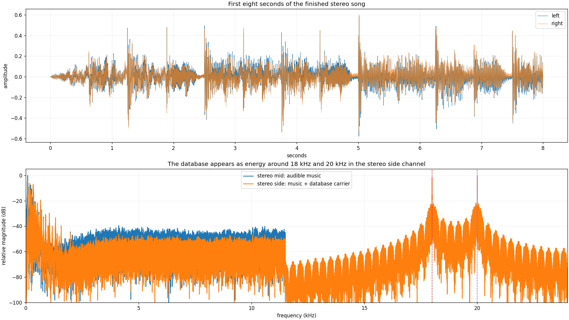
The carrier's RMS level is 19.32 dB below the music RMS, the full song peaks at 0.783 rather than hitting digital full scale, and the carrier begins 2.5 seconds into the track. Those numbers are useful engineering facts, but they are not a fake scientific listenability score; hearing at 18 kHz and 20 kHz varies by person and playback system, so the audio player above remains the honest test.
A small SQLite file is still a real database
The database contains three tables:
| Table | Rows | Purpose |
|---|---|---|
track | 1 | Title, tempo, key, duration, and carrier description |
arrangement | 4 | Section names, start beats, chords, and musical roles |
liner_note | 4 | Notes about composition, encoding, mono failure, and recovery |
SQLite normally stores the complete state of a database in one main file, and its official file-format documentation describes that file as fixed-size pages with a 100-byte header on page one. I set the page size to the minimum supported 512 bytes, created the schema and rows, then ran VACUUM; the result occupies seven pages, or 3,584 bytes.
Those pages contain structure as well as text, so repeatedly deleting vowels from the liner notes would not buy much. I instead compressed the complete file with zlib at level 9. The zlib format in RFC 1950 wraps compressed data with information needed to identify and validate the stream; the database shrank from 3,584 bytes to 867 bytes, a 75.8% reduction.
The source database SHA-256 is:
a59777299e13c94b65532986ac786ca93e8b1ffd73bfb45e1c8a849eb71a2f22SHA-256 is doing comparison here, not secrecy. NIST's Secure Hash Standard defines the algorithm as producing a digest that can be used to detect whether a message changed; the decoder calculates that digest over the recovered database and compares all 32 bytes with the value carried in the packet.
The packet spends redundancy like it is company money
The compressed bytes need enough context to be rejected safely when the audio is damaged. The packet therefore starts with a fixed 51-byte header:
| Field | Bytes | Meaning |
|---|---|---|
Magic value DBSONG1 | 7 | Rejects data that is not this protocol |
| Original length | 4 | Expected database size after decompression |
| Compressed length | 4 | Number of compressed payload bytes |
| SHA-256 | 32 | Exact recovered database identity |
| CRC-32 | 4 | Fast check over the compressed payload |
The 51-byte header plus 867 compressed bytes creates a 918-byte packet. Every packet bit is then repeated three times; the decoder groups each trio and selects the majority, which corrects one wrong symbol inside a group but cannot correct two. A 32-byte alternating preamble and a four-byte sync word sit in front of that repeated body.
The arithmetic is small enough to audit without a protocol analyzer:
prefix       = (32 + 4) * 8             =    288 bits
packet body  = (51 + 867) * 8 * 3       = 22,032 bits
complete frame                            = 22,320 bits
At 1,000 symbols per second, the carrier lasts 22.32 seconds. Repeating everything three times is wasteful, but the whole database already fits; a sophisticated forward-error-correction code would improve efficiency and burst-error handling, while repetition-3 makes the recovery rule visible in four lines of NumPy.
The preamble is currently checked, not searched. The decoder already knows the 2.5-second start time and 1,000-baud symbol rate; a production receiver would scan for the sync sequence, estimate clock drift, and keep tracking timing as the audio changed, but pretending I implemented those pieces would make the reproduction package substantially less funny and the claims substantially less true.
The stereo side channel is the hiding place
Binary frequency-shift keying maps zero and one to two tones. This experiment uses 18 kHz for zero and 20 kHz for one; at a 48 kHz sample rate, each one-millisecond symbol contains 48 samples, 18 cycles of the zero tone, or 20 cycles of the one tone.
The interesting part is where those tones go. If c is the carrier, the encoder applies it with opposite polarity:
left  = music_left  + c
right = music_right - c
Stereo can be represented as mid and side signals:
mid  = (left + right) / 2
side = (left - right) / 2
Substitute the encoded channels and the carrier cancels from the mid signal while adding in the side signal. Normal stereo music remains around it, but the earlier 11.5 kHz low-pass keeps that music away from the two carrier frequencies; the decoder can therefore inspect the side channel and mostly see the data where it expects to see data.
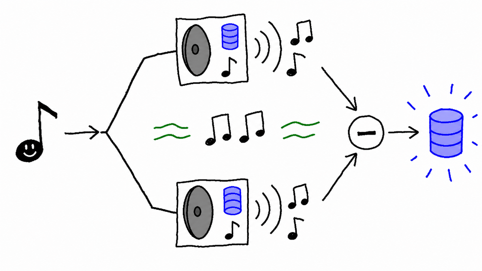
This arrangement also creates an honest failure mode. Converting stereo to mono usually averages left and right; the positive and negative carriers then cancel. The song keeps playing, but its database resigns immediately.
The decoder asks two frequencies one question
The WAV file is written and read with Python's standard wave module, which supports uncompressed PCM. The script converts the generated floating-point mix to 16-bit samples, writes the file, closes it, reopens it, and only then begins decoding; this avoids the wonderfully convenient mistake of proving that pristine in-memory data survived a disk write it never experienced.
For each 48-sample symbol window, the decoder measures energy at both candidate frequencies. It correlates the samples with sine and cosine references, squares and adds those correlations, then calls the symbol a one when 20 kHz has more energy than 18 kHz. Using sine and cosine makes the comparison insensitive to the tone's starting phase within that window.
The remaining recovery path is mechanical:
- Extract
(left - right) / 2from the reopened WAV. - Demodulate all 22,320 binary symbols.
- Compare the 288-bit prefix with the expected preamble and sync word.
- Majority-vote each repeated group of three packet bits.
- Parse the 51-byte header and reject the wrong magic value or lengths.
- Check CRC-32 over the compressed payload, then decompress it.
- Compare database length and SHA-256 with the header.
- Write the recovered bytes as
recovered.sqlite, open them, and run SQLite integrity checks and queries.
The clean WAV produced zero raw bit errors. The recovered file was byte-identical to source.sqlite, and this query worked on the result:
SELECT title, bpm, key, duration_seconds
FROM track
WHERE id = 1;
Side Channel | 96 | C major / A minor | 40.0That is the point where the project stops being a picture of a waveform and becomes a reproducible data channel.
The database survived nine of 12 conditions
I passed the written WAV through 12 deterministic conditions, counted raw demodulated symbol errors before majority voting, and accepted a case only when the recovered database matched the source SHA-256 exactly. The complete machine-readable results live in benchmark.csv.
| Condition | Raw bit errors / 22,320 | Exact database? | Result |
|---|---|---|---|
| Clean WAV | 0 | Yes | Exact recovery |
| Added noise, 50 dB SNR | 0 | Yes | Exact recovery |
| Added noise, 40 dB SNR | 0 | Yes | Exact recovery |
| Added noise, 30 dB SNR | 1 | Yes | Repetition vote corrected it |
| Added noise, 25 dB SNR | 1 | Yes | Repetition vote corrected it |
| Quantized to 12-bit | 0 | Yes | Exact recovery |
| Quantized to 8-bit | 0 | Yes | Exact recovery |
| Clipped at +/-0.35 | 55 | No | Compressed-payload CRC mismatch |
| 12 ms echo at 0.35 gain | 3 | Yes | Exact recovery |
| 48 kHz to 44.1 kHz to 48 kHz | 1 | Yes | Exact recovery |
| 15 kHz low-pass filter | 11,373 | No | Magic mismatch |
| Stereo collapsed to mono | 11,383 | No | Magic mismatch |
Nine exact recoveries out of 12 sounds good, but the numerator is less important than the pattern. The successful cases preserved two distinguishable high-frequency, opposite-polarity tones; the failed low-pass and mono cases explicitly removed them, while severe clipping distorted enough symbols for the packet to fail its CRC.
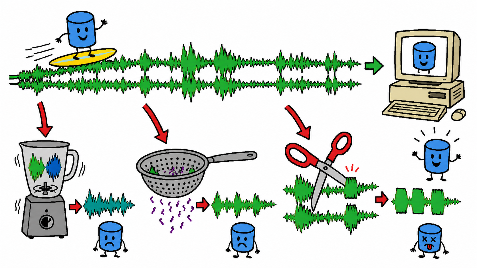
The noise cases use deterministic Gaussian noise measured against the RMS of the whole song. The echo is one delayed copy at 12 ms and 0.35 gain; the resampling case uses linear interpolation down to 44.1 kHz and back, which is simpler than a production sample-rate converter. These are controlled software transformations, not claims about every possible audio pipeline.
The failures explain the mechanism
The mono failure is algebra, not bad luck. Averaging the channels turns +c and -c into zero, so the demodulator receives ordinary music and guesses roughly half the frame incorrectly. This is useful if the goal is to keep the mid signal clean, but terrible if somebody shares the track through a service that normalizes everything to mono.
The 15 kHz low-pass failure is even more direct because both carrier frequencies sit above the cutoff. The output still contains the audible arrangement, yet the data band has been removed; the 50.95% raw error rate is what random guesses look like over this frame.
Clipping is messier. Limiting every sample to +/-0.35 flattens waveform peaks and creates additional spectral energy; the decoder made 55 raw symbol errors, and repetition-3 could not correct every affected group. A changed bit in compressed data can invalidate far more than one output byte, so the CRC rejected the packet before SQLite had to inspect nonsense wearing a .sqlite extension.
The successful 8-bit quantization result looks more surprising, but the detector is only comparing energy at two widely separated frequencies. Coarse sample levels change the waveform while leaving enough of those frequency choices intact; the experiment says this one deterministic quantizer survived, not that all low-bit audio conversions are safe.
What this does not prove
This is not encryption. The database, protocol, frequencies, and code are public; anybody who extracts the payload can read the tables. It is also not strong steganographic secrecy because a spectrum plot makes the 18 kHz and 20 kHz energy rather obvious. The carrier is better described as data hidden from casual listening than data hidden from an analyst.
The decoder has known timing. It begins exactly 2.5 seconds into the file, expects 1,000 symbols per second, and does not search for time stretching or drift; trimming the intro, changing playback speed, or recording the track through a speaker would require synchronization and channel-estimation work that this version does not implement.
I did not test MP3, AAC, Opus, streaming normalization, a phone speaker-to-microphone loop, room acoustics, or Bluetooth transcoding. Lossy codecs often make their own decisions about high-frequency content, but the only defensible result here is that those pipelines remain untested. A future version should sweep codec settings and run physical loopback trials rather than converting that suspicion into a pretend benchmark.
Finally, "decent song" is a human judgment. The artifact has a progression, rhythm section, lead, variations, controlled peak level, and a carrier measured 19.32 dB below the music RMS; those are reproducible properties, while whether the result belongs on your playlist is why the WAV is embedded near the top.
Questions people will reasonably ask
Is hiding a database in a song audio steganography?
It is a small audio data-hiding experiment and fits the broad idea of audio steganography, but it is not covert against inspection. The payload sits at fixed high frequencies with opposite stereo polarity, and the public decoder knows exactly where to look; a spectrum or side-channel plot gives the trick away quickly.
Does the database survive MP3 or streaming compression?
That remains untested. The experiment covers PCM quantization, additive noise, echo, linear resampling, clipping, low-pass filtering, and mono collapse; it does not claim survival through MP3, AAC, Opus, or a streaming platform. Those codecs can alter high-frequency content, so each codec and bitrate needs its own measured result.
Can SQLite query the WAV directly?
No. The decoder first reconstructs the exact SQLite file from the audio samples, then SQLite opens that recovered file normally. Teaching SQLite to treat a WAV as a virtual file system would be a separate and deeply unnecessary sequel.
How much data can fit inside a song this way?
This frame carries 867 compressed payload bytes in 22.32 seconds because every packet bit is repeated three times and the channel runs at 1,000 symbols per second. A longer song, higher symbol rate, more carrier frequencies, or stronger coding scheme could change the capacity; each option also changes audibility, error tolerance, bandwidth, and decoder complexity, so the useful answer is a tradeoff curve rather than one impressive number.
Reproduce the song and database
The experiment directory contains the complete composer, database builder, packet encoder, WAV writer, decoder, benchmark, source and recovered databases, rendered song, manifest, and first-party spectrum plot. It uses Python's standard library plus pinned NumPy and Matplotlib versions.
On Windows:
cd public\research\database-song
python -m venv .venv
.\.venv\Scripts\python.exe -m pip install -r requirements.txt
.\.venv\Scripts\python.exe run_experiment.py
On macOS or Linux, use .venv/bin/python for the final two commands. A passing run creates the artifacts under outputs/, decodes side-channel.wav, checks the exact hash and SQLite integrity, executes all 12 benchmark cases, and writes the same measurements used in this article to manifest.json.
If you only want to audit the published outputs without regenerating the composition, the standalone verifier uses the Python standard library:
python verify_artifact.pyIts expected summary is:
Side Channel artifact verified
  WAV: 2 channels, 48000 Hz, 16-bit PCM, 40.00 s
  SQLite SHA-256: a59777299e13c94b65532986ac786ca93e8b1ffd73bfb45e1c8a849eb71a2f22
  PRAGMA integrity_check: ok
  Recovered title: Side Channel
  Benchmark: 9/12 exact recoveries
  Intentional failure modes: clipped_0_35, lowpass_15khz, mono_collapse
The next technically interesting upgrade is not a larger database; it is a receiver that finds the frame without knowing its start time, tracks clock drift, and then measures survival through real codecs and a physical room. The current version stays small enough that every step from SQL row to audio sample and back can be read in one file.
Sources and artifacts
- Live Web Audio side-channel lab
- Complete reproducible experiment package
- Composer, database builder, encoder, decoder, and benchmark
- Standalone artifact verifier
- Machine-readable manifest and recovery summary
- Raw 12-case benchmark
- SQLite database file format
- SQLite PRAGMA integrity_check
- RFC 1950: zlib compressed data format
- NIST FIPS 180-4 Secure Hash Standard
Conclusion
This song really has a database in it. A 3,584-byte SQLite file becomes an 867-byte compressed payload, a 918-byte packet, and 22,320 high-frequency symbols carried for 22.32 seconds inside a 40-second stereo track; the decoder reads the finished WAV, recovers every source byte, matches SHA-256, receives ok from SQLite, and returns the song's own metadata and liner notes.
The broader engineering lesson is that a ridiculous demo becomes useful when its boundaries are specific. "Data in audio" is a vibe; a documented packet, exact hash, database integrity check, raw benchmark, playable artifact, and three intentional failures make it a result. The narrower lesson is that converting the song to mono fires the database, so please respect its employment contract.